Mastering Probability: Your Ultimate Guide to the Binomial Probability Distribution Calculator

Have you ever wondered about the chances of a specific outcome in a series of events? What are the odds of getting heads five times in ten coin flips? Or how many defective products you might find in a batch of 100? These questions are at the heart of probability, a branch of mathematics that helps us understand uncertainty. While the concepts can seem complex, a powerful tool can make them surprisingly simple: a binomial probability distribution calculator.

This guide will walk you through a comprehensive probability suite, designed to demystify everything from basic chances to more advanced calculations. We will explore how this versatile tool, especially its function as a binomial probability distribution calculator, can help you solve real-world problems. Whether you’re a student, a professional in quality control, or just curious about how probability works, this resource will break down the essentials in an easy-to-understand way. We’ll cover everything you see on the screen, from input fields to the final charts, making you a probability expert in no time.

A First Look at the Probability Suite

When you first open this probability tool, you’ll notice a clean, user-friendly interface. It’s designed to be intuitive, even if you’ve never touched a probability formula before. The layout is organized into distinct sections, making it easy to find exactly what you need.

At the top, you’ll see a series of tabs: Basic Probability, Combinations (nCr), Permutations (nPr), and Binomial Probability. This modular design allows you to tackle different types of probability problems one at a time. Each tab presents a specialized calculator for that specific concept. Below the tabs, the main content area changes depending on which calculator you’ve selected, showing you the right input fields, buttons, and result displays. This entire suite serves as a fantastic binomial probability distribution calculator and much more.

The visual design is clear, with bold headings, well-defined input boxes, and a prominent “Calculate” button. This ensures you know exactly where to enter your numbers and how to get your answer. The results are not just a single number; they are often presented in detailed boxes, with step-by-step explanations and even graphical charts to help you visualize the data. This commitment to clarity makes it more than just a calculator—it’s a learning tool.

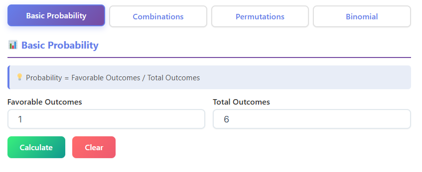
Diving into the Basic Probability Tab

Your journey into probability begins with the fundamentals, and the Basic Probability tab is the perfect starting point. This section helps you calculate the likelihood of a single event happening.

Understanding the Inputs

On this tab, you are greeted with two simple input fields:

1. Number of Favorable Outcomes: This is where you enter the number of ways your desired event can occur. For example, if you want to find the probability of rolling a 4 on a standard six-sided die, there is only one favorable outcome (rolling a 4).
2. Total Number of Possible Outcomes: Here, you enter the total number of results that could happen. For our six-sided die, there are six possible outcomes (1, 2, 3, 4, 5, or 6).

After filling in these two boxes, you click the “Calculate” button. The tool instantly processes your information and displays the results.

Interpreting the Results

The results are presented in a clear and organized manner, showing the probability in four different formats:

• Fraction: This shows the probability as a simple fraction (e.g., 1/6).
• Decimal: The fraction is converted into a decimal format (e.g., 0.1667).
• Percentage: The probability is expressed as a percentage (e.g., 16.67%).
• “1 in X” Chance: This format makes the probability very intuitive. For our die roll, it would tell you that you have a “1 in 6” chance of rolling a 4.

This section is a great warm-up, building your confidence before you move on to more complex scenarios and the powerful binomial probability distribution calculator feature.

Understanding Order with Permutations (nPr)

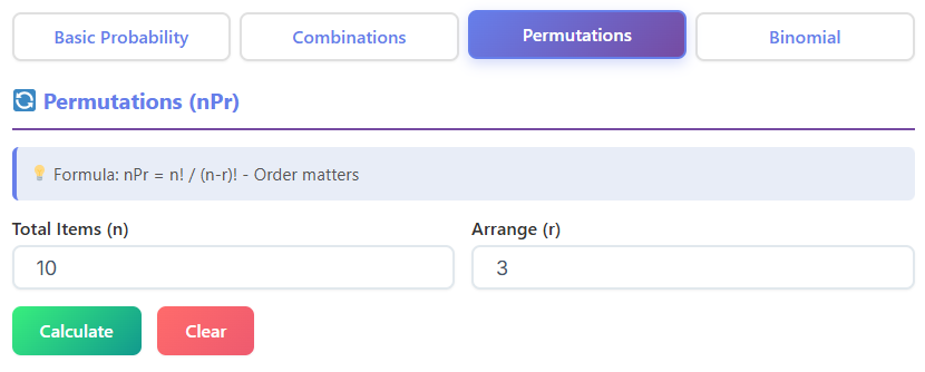
Next up is the Permutations (nPr) tab. Permutations are about arrangements where the order of items matters. Think about arranging books on a shelf or determining the first, second, and third place winners in a race.

The Inputs for Permutations

This calculator requires two values:

1. Total Number of Items (n): This is the total size of the set you are choosing from. For example, if you have 8 people in a race, n = 8.
2. Number of Items to Arrange (r): This is the number of items you are selecting and arranging. If you want to find the number of ways to award gold, silver, and bronze medals, r = 3.

Once you enter these values and click “Calculate,” the tool computes the number of possible permutations.

Making Sense of the Permutation Results

The output is straightforward. A result box will show you the total number of permutations. For our race example (8 people, 3 medals), the answer would be 336. This means there are 336 different ways to award the top three prizes.

Below the answer, you’ll find the Permutation Formula (nPr) displayed: P(n,r) = n! / (n-r)!. The tool doesn’t just give you the answer; it shows you the formula used to get there. This helps you understand the mathematical logic behind the result. The factorial symbol (!) means multiplying a number by all the positive whole numbers less than it (e.g., 4! = 4 x 3 x 2 x 1). This tab is a crucial stepping stone toward understanding the more advanced binomial experiment formula.

Exploring Combinations (nCr) Where Order Doesn’t Matter

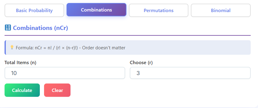
The Combinations (nCr) tab is similar to permutations, but with one key difference: order does not matter. This is for situations where you are selecting a group of items, and the arrangement within the group is irrelevant. Think about picking a team of 3 players from a group of 10, or choosing 5 toppings for a pizza.

Combination Calculator Inputs

The inputs are the same as for permutations:

1. Total Number of Items (n): The size of the entire pool you are choosing from.
2. Number of Items to Choose (r): The size of the subgroup you are selecting.

Let’s say you want to know how many different 5-card hands you can get from a standard 52-card deck. Here, n = 52 and r = 5.

Understanding the Combination Results

After clicking “Calculate,” you get a single number representing the total possible combinations. For the 5-card hand example, the result is 2,598,960.

Just like the permutations tab, this section also displays the formula used: Combination Formula (nCr), C(n,r) = n! / (r!(n-r)!). Seeing this helps you appreciate why the number of combinations is usually smaller than the number of permutations. By dividing by an extra r!, we remove all the duplicate arrangements. This concept of choosing a certain number of successes from a number of trials is fundamental to using a binomial probability distribution calculator.

The Main Event: The Binomial Probability Distribution Calculator

Now we arrive at the most powerful feature of this tool: the Binomial Probability tab. This section is a complete binomial probability distribution calculator designed to handle more complex probability questions. A binomial distribution applies to scenarios that meet four criteria:

1. There are a fixed number of trials (e.g., flipping a coin 10 times).
2. Each trial is independent of the others.
3. Each trial has only two possible outcomes (e.g., heads/tails, success/failure, pass/fail).
4. The probability of success is the same for each trial.

This is where the real power of a binomial distribution calculator shines.

Inputs for the Binomial Probability Distribution Calculator

The interface on this tab is more detailed, but still very clear. You’ll need to provide the following information:

1. Probability of Success (p): This is the probability of success on a single trial, expressed as a decimal. For a fair coin, the probability of getting heads is 0.5. For a quality control check where 2% of items are defective, the probability of finding a defective item is 0.02.
2. Number of Trials (n): This is the total number of times the event is repeated. For example, flipping a coin 10 times means n = 10.
3. Number of Successes (x): This is the specific number of successes you are interested in. You can ask for the probability of exactly a certain number of successes, at most a number, or at least a number.

Let’s use a practical example. A factory produces light bulbs, and 5% of them are defective. You randomly sample 20 bulbs. What is the probability that exactly 2 of them are defective?

• Probability of Success (p) = 0.05 (Success here is defined as finding a defective bulb)
• Number of Trials (n) = 20
• Number of Successes (x) = 2

Once you enter these values into the binomial probability distribution calculator and click “Calculate,” you unlock a wealth of information.

Deconstructing the Results

The results from the binomial probability distribution calculator are incredibly thorough, giving you a full picture of the scenario.

The Main Probability Results

At the top, you’ll see the key probabilities calculated for you:

• P(X = x): The probability of getting exactly x successes. In our light bulb example, this would be the probability of finding exactly 2 defective bulbs.
• P(X < x): The probability of getting fewer than x successes.
• P(X ≤ x): The probability of getting at most x successes (less than or equal to).
• P(X > x): The probability of getting more than x successes.
• P(X ≥ x): The probability of getting at least x successes (greater than or equal to).

Each of these results provides a different perspective on the problem, allowing you to answer a wide range of questions with a single calculation. This comprehensive output is a hallmark of a great binomial probability distribution calculator.

The Binomial Experiment Formula Box

Just below the main results, the tool shows you the binomial experiment formula: P(X=x) = C(n,x) * p^x * (1-p)^(n-x). Let’s break down what this means in simple terms:

• C(n,x): The number of ways to choose x successes from n trials (which you learned about in the Combinations tab).
• p^x: The probability of getting x successes.
• (1-p)^(n-x): The probability of getting n-x failures.

Seeing the formula with your numbers plugged in reinforces your understanding. You can see exactly how the binomial probability distribution calculator arrived at the answer, turning a black box into a transparent learning process. This feature makes it more than a simple binomial distribution calculator; it’s an interactive textbook.

The Step-by-Step Solution Box

For even greater clarity, a “Show Steps” button often reveals a step-by-step breakdown of the calculation. It walks you through:

1. Identifying the values of n, p, and x.
2. Calculating the combinations part, C(n,x).
3. Calculating the success probability part, p^x.
4. Calculating the failure probability part, (1-p)^(n-x).
5. Multiplying them all together to get the final probability.

This feature is invaluable for students who need to show their work or for anyone wanting to truly master the binomial experiment formula. It confirms that the binomial probability distribution calculator is following the correct mathematical procedure.

Key Metrics and Distribution Properties

A good binomial probability distribution calculator also provides summary statistics about the entire probability distribution. You’ll typically see a box with these metrics:

• Mean (μ): The expected or average number of successes, calculated as μ = n * p. For our light bulb example, the mean would be 20 * 0.05 = 1. This means that on average, you can expect to find 1 defective bulb in any sample of 20.
• Variance (σ²): A measure of how spread out the data is, calculated as σ² = n * p * (1-p). A smaller variance means the outcomes are likely to be very close to the mean.
• Standard Deviation (σ): The square root of the variance. It’s a more intuitive measure of spread, expressed in the same units as the data.

These metrics provide a high-level overview of your binomial experiment without needing to calculate each individual probability. Understanding these metrics is a key part of using a binomial probability distribution calculator effectively.

Visualizing the Data: The Binomial Curve

One of the most powerful features of a top-tier binomial probability distribution calculator is its ability to generate a chart of the results. This chart, often a bar graph, represents the full binomial probability distribution.

Each bar on the graph corresponds to a possible number of successes (from 0 to n). The height of each bar represents the probability of achieving that specific number of successes. This visual representation is known as the binomial curve (or more accurately, a binomial distribution histogram).

What the binomial curve shows you:

• The Shape of the Distribution: You can see if the distribution is symmetric (which happens when p=0.5) or skewed. If p is low, the curve will be skewed to the right, with most outcomes clustered at lower numbers of successes. If p is high, it will be skewed to the left.
• The Most Likely Outcome: The tallest bar on the graph corresponds to the mean or expected value, showing you the most probable result of your experiment.
• Probability at a Glance: You can visually compare the likelihood of different outcomes. For instance, you can see that the probability of finding 10 defective bulbs in our example would be extremely low, as its bar would be almost invisible.

The chart often highlights the bar corresponding to your chosen x, making it easy to see where your specific query falls within the overall distribution. This visual feedback is what makes a sophisticated binomial probability distribution calculator an indispensable learning aid. The binomial curve transforms abstract numbers into a tangible shape, making probability feel much more intuitive.

Practical Examples in Action

Let’s see how this multi-functional binomial probability distribution calculator can be applied to solve everyday problems.

Scenario 1: Coin Flips

You flip a fair coin 15 times. What is the probability of getting exactly 8 heads?

• Go to the Binomial Probability tab.
• Probability of Success (p): 0.5 (chance of heads)
• Number of Trials (n): 15
• Number of Successes (x): 8
• The binomial probability distribution calculator would instantly tell you the probability P(X=8). You could also see the probability of getting at least 8 heads or at most 8 heads, and view the entire binomial curve for 15 flips.

Scenario 2: Multiple-Choice Test

You are taking a 20-question multiple-choice test. Each question has 4 options, and you guess on every single one. What is the probability you pass if passing is 60% (12 questions correct)?

• This is a binomial problem. For each question (trial), you either get it right (success) or wrong (failure).
• Probability of Success (p): 0.25 (1 correct option out of 4)
• Number of Trials (n): 20
• Number of Successes (x): You need to find the probability of getting at least 12 correct. So you’re interested in P(X ≥ 12).
• The binomial probability distribution calculator will calculate this for you. You would enter p=0.25, n=20, and x=12. Then you would look at the result for P(X ≥ 12). The answer would likely be very, very small, illustrating why guessing is not a good strategy! This is a perfect job for a reliable binomial probability distribution calculator.

Scenario 3: Marketing Campaign

A marketing team sends out 1,000 promotional emails. Historically, 10% of these emails are opened. What is the probability that at least 120 people open the email?

• Probability of Success (p): 0.10
• Number of Trials (n): 1000
• Number of Successes (x): 120
• Using the binomial probability distribution calculator, you would find P(X ≥ 120). This information could help the marketing team set realistic expectations for their campaign. The binomial curve would show them the most likely range of opens.

In each case, the binomial distribution calculator simplifies a complex problem into a few simple inputs and provides a rich, detailed output.

Why This Tool is More Than Just a Calculator

Throughout this guide, we’ve explored the various tabs and features of this comprehensive probability suite. From basic probabilities to complex arrangements and binomial scenarios, the tool is designed to be your all-in-one resource. It’s more than just a way to get quick answers; it’s an interactive learning platform.

By showing the formulas, breaking down the steps, providing key metrics, and visualizing the data with the binomial curve, the tool empowers you to understand the why behind the what. It builds your confidence and deepens your knowledge of probability.

The seamless integration of a combinations calculator, a permutations calculator, and a premier binomial probability distribution calculator makes it an essential asset for anyone working with statistics. Whether you are a student trying to ace an exam, a quality assurance engineer monitoring production lines, or a researcher analyzing experimental data, this binomial probability distribution calculator gives you the power to make informed, data-driven decisions. It turns abstract mathematical concepts into practical, applicable insights. This binomial probability distribution calculator is your key to unlocking the world of probability.

FAQs